That was a really good interview, hats off to both of you for putting the numbers out there. I’ll have to give it an audio re-listen on a long drive I have tomorrow.
I’m going to throw in some data and fits that I’ve been holding back for a while. It more or less jibes with Adam’s group’s analysis. Since the EIA went bonkers last year and started including natural gas liquids in their total petroleum numbers, there’s no more unpolluted data easily available and I’ve dropped out of the production prediction game. But here’s as far as I got.
edit: Note, this is all for domestic US production. May not have made that clear in the rest of the text.
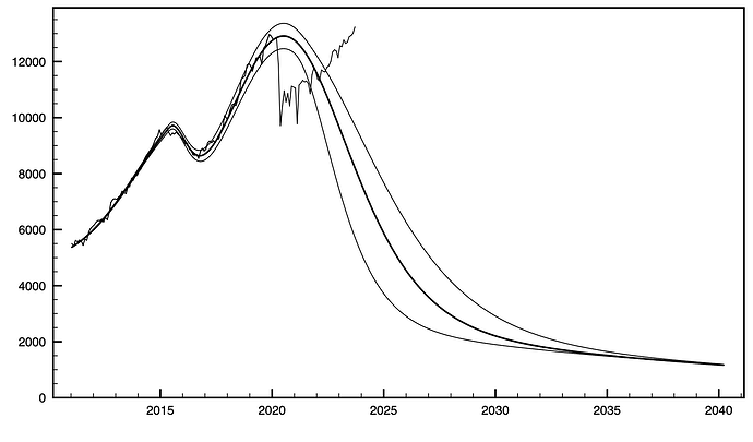
What you see here is a fit of four logistic distributions to EIA US oil production data, going back to 1920. The fitting engine is a genetic algorithm, using statistical error weighting on the data. NB, these are not the same as normal (i.e.Gaussian) distributions. Though they are qualitatively similar, they have thicker tails. Here’s a link to the wiki on these: Logistic distribution - Wikipedia They’re commonly used to describe saturation and depletion phenomena, and BTW they do a decent job of modeling uncontrolled disease spread numbers.
The width parameter (s in the linked article’s nomenclature) was allowed to have different values on the two sides of each peak. This allows for “Seneca cliff” behavior in the fitted curves. Four peaks (conventional CONUS, Alaska, and two for fracked oil), and four parameters each. There were a handful of other standard numerical techniques used that I won’t further bore the audience with.
The down-side width for the fourth peak could not be determined, simply because it hasn’t happened yet so there is no data. The up-side width was used to make the plot. Alternately, if the total recoverable oil numbers were available, we could integrate under the curves to come up with the downside-s. However, the total recoverable reserve numbers are (a) not easily available, and (b) not all that accurate.
FWIW, the down-s for the first tight oil peak is about 1/3rd the value for the upside-s — one hell of a Seneca cliff! Also, these widths were about 1/20th the values for the CONUS conventional and Alaska peaks. Be afraid.
Also, the fits are only to data thru early 2020. The production numbers went crazy after that. We might have recovered from that glitch, but now the data’s been muddied since last year with the inclusion of the natural gas liquids into the petroleum production numbers. Not worth the bother of fitting: garbage in, garbage out.
The uncertainty bounds are one standard deviation of the results from the GA’s population ensemble results, for the last peak only. It’s as good a method as any, but that’s another discussion.
Logistic distros are a stone cold bitch to fit. A semi-log plot (not shown) reveals why. During the main growth and decline phases they are nearly linear (i.e., exponential on a linear plot), and have little curvature to give a hint as to when the peak production year will occur. Even though we’re fitting linear data, this underlying behavior persists. In contrast, normal distros are inverted parabolas on a semi-log plot, have plenty of curvature from which to extract some future peak date, and are real sweethearts for numerical fitting. That’s why they’re used so often!
BTW, Hubbert used a data linearization process, and then did a linear fit to that. In the mid-50’s he predicted a peak around 1967. Using the method described above (with just one peak) on the data available to Hubbert at the time, 1970 was predicted, smack on what it turned out to be. For the algorithms and computing power available at the time, Hubbert did a remarkable job.
Normal distros have their uses in fitting oil peaks too. I’ve had fair results using these on world oil production figures, better than with logistic distros. With all the production interruptions from wars, regime changes, and bad data, the central limit theorem kicks in and the individual logistic distros blur into normals. But the data’s all crap, and I can’t really draw much from it. For domestic production though, things are orderly enough that logistic distros do better.
OK, so all that said, here are my conclusions:
(1) We’re screwed.
(2) The numbers since about 2021 are being juiced, probably to make the powers that be look good.
(3) Adding in the natural gas liquids is just dirty pool, and makes further predictions from the EIA gross data nearly impossible…
(4) But they can’t keep the number manipulation going forever.
(5) I would NOT want to be the occupant of White House circa 2026, when the decline really gets rolling and is no longer concealable.
(6) When the fracked oil is gone, things kind of level out circa 2030 on conventional oil’s longer tail at about 20% of peak production. Maybe Pareto’s principle will help out as the pain sets in, and we won’t be quite as screwed as this seems at first look. More of “muddling through,” like the 70’s malaise on steroids.
(7) Over the following decade up to 2040, that 20% will drop to maybe 12% of the peak at a comparatively gentle rate. That’ll give us time to get serious about either nuclear power or breeding more draft animals. Because it’s going to be one or the other, choose wisely.
Now that I’ve gotten that off my chest, off to bed. Really good interview, can’t wait to give it a thorough second go-through tomorrow.


